Few-step text generationwith Inverse Distillation

1. Motivation

1.1 General Approaches: Autoregression vs Diffusion

Most modern language models use the autoregressive recipe behind Transformers and GPT-style models: generate one token, append it to the context, then generate the next token. This gives a clean probabilistic factorization,

This is why autoregression is so strong in text: training is stable, causal transformers scale well, and sampling decisions are easy to interpret. The price is the sampling loop. A \(L\)-token completion usually needs \(L\) sequential forward passes, because token \(i\) cannot be sampled before token \(i-1\) exists.

Diffusion language models use a different generation view. They start from a noisy sequence and repeatedly denoise it, so each denoising call can look at the whole sequence and revise many token positions together. Recent models such as D3PM, MDLM, SEDD, UDLM, and LLaDA show that this bidirectional, whole-sequence paradigm can be competitive for language. The promise is not that one denoising call magically solves generation. The promise is that the expensive sequential dimension might move from sequence length to the number of denoising rounds.

Autoregressive

Diffusion

1.2 The Problem of Diffusion Inference

Despite their strong potential for high-quality generation, diffusion models retain a central practical limitation: inference is slow. A sampler starts from noise and repeatedly calls the denoising network, call \(k\) consumes the output of call \(k+1\). So even though one call can update all tokens in parallel, the outer loop may require \(50\), \(100\), \(250\), or \(1000\) forward passes before the sequence becomes clean.

The natural acceleration idea is to replace many small denoising steps with a few large jumps. But the reverse transition used by many discrete diffusion models is factorized over positions:

This works well when the jump from \(x_t^{1:L}\) to \(x_{t-1}^{1:L}\) is small: most sentence structure is already present, and each token only needs a local correction. A large skip from \(x_t^{1:L}\) to \(x_{t-\Delta}^{1:L}\) asks one factorized transition to capture stronger cross-token dependencies:

This is the central tension. A composition of many small factorized transitions can still represent a rich final distribution, because later steps can repair earlier local mistakes. If we remove most of those steps, one factorized jump must suddenly coordinate agreement, syntax, semantics, and long-range dependencies. That is where naive step-skipping becomes fragile.

Large factorized jump Correlation can break

Independent choices can create incompatible tokens, for example cat with are.

Many small steps Small errors get repaired

A short correction can use the partially cleaned context before choosing the next token.

1.3 Distillation in Image Diffusion

Image diffusion made this tradeoff visible before language diffusion did. Models such as DDPM, score-based SDEs, and EDM showed that a noisy sample can be transformed into a high-quality image by following a reverse denoising process. In DDPM this process is a long reverse Markov chain, in score-based SDEs it can be viewed as integrating a reverse-time stochastic or deterministic dynamics.

The cost is that each reverse step requires another neural network evaluation. The original DDPM-style samplers commonly used very long chains, while accelerated samplers such as DDIM and Improved DDPM reduced the number of evaluations but did not remove the sequential nature of sampling. This is why image diffusion became the natural testbed for distillation: if a student can replace many small denoising moves with a few reliable jumps, we can keep most of the teacher's visual quality while paying for far fewer forward passes.

Image diffusion generation \(T\) sequential denoising steps

Input noise

Step \(1\) Denoising model

Step \(2\) Denoising model

Step \(3\) Denoising model

...

Step \(T-1\) Denoising model

Step \(T\) Denoising model

Distillation changed that story by asking a sharper question: can we keep the distribution learned by a strong teacher while reducing the number of sequential denoising calls? Progressive distillation, for example, trains a student sampler to imitate multiple teacher steps with one larger step, then repeats this compression. Consistency models learn a shortcut from points along a diffusion trajectory back to the clean sample, which makes one-step or few-step generation possible. This idea was later scaled in systems such as latent consistency models. A complementary line, distribution matching distillation (DMD), directly trains the student distribution to match the teacher-supported data distribution, rather than only copying local transitions.

The lesson from image diffusion is that acceleration is not only a faster sampler, it is a training problem. The student must take larger jumps without drifting away from the teacher's distribution. This is the motivation for IDLM: keep the parallel, bidirectional view of language diffusion, but transfer the successful distillation idea into the discrete text domain, where tokens are not continuous pixels, gradients cannot flow through token choices in the same way, and large factorized jumps can break cross-token structure.

Distilled image diffusion \(k\) student denoising steps, \(k \ll T\)

Input noise

Step \(1\) Student denoiser

Step \(2\) Student denoiser

Step \(3\) Student denoiser

Step \(k\) Student denoiser

2. Inverse Distillation

2.1 Two General Distillation Approaches

Continuous diffusion distillation is often organized into two families. The first is consistency-like distillation. A teacher provides a denoising trajectory, and the student learns to map different points on that trajectory to a consistent clean output. In plain terms, it teaches the model to skip along the path. This idea is powerful and relatively direct, and discrete-language variants such as SDTT and Duo-DCD show that trajectory-shortening can help diffusion language models too.

The second is distribution-matching distillation. Here we directly parameterize a student distribution \(p_\theta\) and train it to match the teacher-supported data distribution \(p^\star\). Image methods such as DMD do this with an auxiliary model that estimates whether the current student distribution matches the teacher distribution. This view is usually more involved, because the auxiliary model must be trained while the student changes, but the target is stronger: match the distribution, not merely a local denoising shortcut.

2.2 The Inverse Distillation View

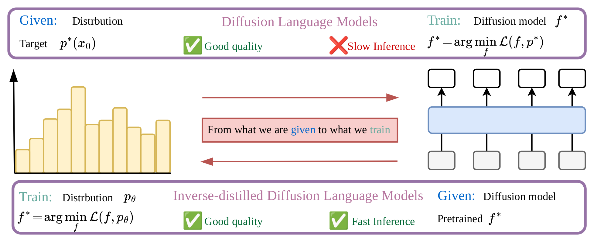
Inverse Distillation is a distribution-matching-style distillation approach. The goal is to train a fast student distribution \(p_\theta\) so that it matches the target data distribution \(p^\star\). The central question is how to compare \(p_\theta\) with \(p^\star\). Inverse distillation answers this by comparing the diffusion models that would be learned from these two distributions.

First recall the ordinary, or forward, diffusion-training problem. We start with real data samples \(x_0 \sim p^\star\), corrupt them with the prescribed noising process, and learn a reverse denoising model by minimizing a diffusion training loss \(\mathcal{L}\). In the notation below, the optimal diffusion model \(f^\star\) trained on \(p^\star\) satisfies:

Inverse distillation reverses this relationship. Instead of asking which diffusion model is optimal for a known distribution, we are given the already-trained teacher \(f^\star\) and ask which student distribution \(p_\theta\) would make this same teacher optimal. A perfect student should therefore satisfy the inverse optimality condition

This condition says more than "move samples toward the teacher." It says that if we took samples from the current student \(p_\theta\), noised them, and trained a diffusion model with the same loss, the model recovered by this training procedure should be \(f^\star\). In practice, we approximate this test with a second, learnable diffusion model \(f\), often called the fake model. This fake model is trained on the current student samples, so it represents the best diffusion model that the student distribution itself can explain.

The inverse-distillation loss then compares two denoisers on the same student distribution: the frozen teacher \(f^\star\), which encodes the target \(p^\star\), and the fake model \(f\), which is optimized for the current \(p_\theta\). Minimizing the resulting teacher-minus-fake gap encourages \(p_\theta\) to become a distribution for which the teacher is already the optimal diffusion model:

If the inverse problem is solved perfectly, the generator recovers the same data distribution that produced the teacher. This inverse-distillation line started from Inverse Bridge Matching Distillation, was extended by Universal Inverse Distillation, and was further clarified by Residual Shifting Distillation in relation to DMD-like objectives. In continuous domains, this gives both a theoretical uniqueness story and practical few-step generators.

2.3 From Images to Language

Of course, we would like to transfer this inverse-distillation principle to the language domain: start from a strong pretrained diffusion language model, train a faster student distribution \(p_\theta\), and preserve the same distribution-matching interpretation. However, language introduces difficulties that are absent, or much less severe, in the continuous image setting. The main obstacle is that text lives on a discrete token space. A token is a categorical state, not a point that can be moved infinitesimally along a smooth pixel-space direction.

This discreteness creates an optimization problem. If the student generator outputs hard one-hot tokens, the mapping from logits to tokens is non-smooth, and gradients cannot pass through the sampling decision in the usual way. One can relax a token into a probability vector on the simplex, which makes the generator output differentiable, but this introduces a second problem: the pretrained teacher was typically trained on hard token states. As a result, evaluating the teacher on relaxed intermediate states may produce unstable or poorly calibrated training signals. Thus, simply copying the continuous inverse distillation recipe into language is not mathematically or practically sufficient.

There is also a sequence-level issue. A language model should not generate a sentence by choosing \(64\) tokens independently. The tokens must agree with one another: they must maintain topic, syntax, agreement, discourse structure, style, and long-range semantic dependencies. In other words, the object to be matched is not only a collection of token-wise marginals, but a distribution over coherent sequences. A valid language distillation objective must therefore preserve the distribution-matching promise of inverse distillation while remaining differentiable, well-defined for discrete diffusion processes, and sensitive to sequence-level structure. This is the role of IDLM.

Continuous

smooth

Discrete

3. IDLM: Inverse-distilled Diffusion Language Models

3.1 Theoretical Guarantees

The first contribution of IDLM is to make the inverse-distillation objective well posed for discrete diffusion. Let \(p^\star\) denote the target distribution over clean token sequences, and let \(p_\theta\) be the distribution produced by the student generator \(G_\theta\). The frozen teacher \(f^\star\) is the diffusion model trained on \(p^\star\), while \(f\) is a fake diffusion model trained on samples from \(p_\theta\). With \(\mathcal{L}(f,p)\) denoting the diffusion loss for model \(f\) when the clean samples come from distribution \(p\), IDLM optimizes the inverse gap \(\mathcal{L}(f^\star,p_\theta)-\min_f \mathcal{L}(f,p_\theta)\).

In a discrete space, this gap is not automatically meaningful: a poorly chosen objective could have minimizers that do not recover the data distribution. The theorem shows that for the losses underlying SEDD, MDLM, and Duo in the hard-token limit, the ideal IDLM objective has the desired unique zero-loss solution:

Here \(D_{\mathrm{KL}}(p_\theta \Vert p^\star)\) measures the mismatch between the final clean distributions. Therefore the inequality says something stronger than non-negativity: if the IDLM loss goes to zero, then the student distribution itself must converge to the target distribution. This rules out the most dangerous failure mode, where the student satisfies the inverse objective but still generates from the wrong clean distribution.

The proof also explains why the objective has this property. For a clean distribution \(p\), run the corresponding discrete diffusion process and look at the entire stochastic trajectory, not just the endpoint. Let \(\mathbb{P}^{\star}\) be the path distribution induced by \(p^\star\), and let \(\mathbb{P}^{\theta}\) be the path distribution induced by \(p_\theta\). If we could compute the losses exactly, the IDLM objective would be the KL divergence between these full trajectory distributions:

This path-level view is the key difference from marginal-matching distillation. If \(p_t^\theta\) and \(p_t^\star\) are the noised marginals obtained at diffusion time \(t\) from \(p_\theta\) and \(p^\star\), a DMD-like objective compares these marginals time by time:

where \(w(t)\) is a time-dependent weight. This checks whether the student and teacher look similar at sampled noise levels, but it does not directly compare how probability mass moves across the whole reverse chain. IDLM instead compares the joint law of the full path, so the objective keeps information about the coupling between consecutive states. A stop-gradient simplification can make the IDLM update resemble a DMD-style marginal update, but that is not the full inverse-distillation gradient. For MDLM, the \(\mathrm{SUBS}\) parameterization hides part of this distinction because already revealed tokens are copied and contribute zero loss. For uniform diffusion, tokens can be revised repeatedly, so the path dependence remains visible and becomes important for stable optimization.

3.2 Handling Discrete Non-Smoothness

In practice, IDLM does not store the student distribution \(p_\theta\) explicitly. It represents it with a generator \(G_\theta\): sample a latent variable \(\epsilon\), pass it through \(G_\theta\), and obtain a candidate clean sequence. The difficulty is that text is discrete. If the generator immediately samples or chooses a hard one-hot token, the map from its logits to the token is no longer smooth, so the IDLM loss cannot send a useful gradient back into \(G_\theta\).

IDLM therefore trains the generator in a relaxed space. For each token position, \(G_\theta(\epsilon)\) outputs a probability vector on the vocabulary simplex: all entries are nonnegative and sum to one. This vector is still a valid distribution over words, but it is differentiable with respect to the generator parameters. The teacher and fake diffusion losses can then evaluate soft token probabilities during training, and their difference can flow back through the simplex vector to update \(G_\theta\). At sampling time, the model can still turn these probabilities into actual discrete tokens.

Masked diffusion gives IDLM an important shortcut. In the \(\mathrm{SUBS}\) parameterization, a token that has already been revealed is treated as fixed: later reverse transitions simply copy it forward rather than resampling it. As a result, the teacher model \(f^*\) and the fake model \(f\) make the same prediction on these copied coordinates. Their loss difference cancels there, so the useful IDLM signal is concentrated exactly on the positions that remain masked and still need to be predicted.

This is why IDLM-MDLM can use a clean mask-only update: it does not need to differentiate through every sampled intermediate token in the reverse chain. Uniform diffusion does not have this copy-once structure. A position can move from one token to another across multiple reverse steps, so the training signal depends on the whole path through intermediate categorical states. IDLM therefore uses the Duo relaxation to replace hard token samples with differentiable simplex states during training. This keeps gradients flowing through the intermediate transitions, which is essential when the model must learn both what token should appear and how the reverse process should move toward it over time.

3.3 Sequence-Level Generative Capacity

How can a generator produce coherent text if the generator still produces a product over token positions? The answer is that the product is conditional, not marginal. IDLM views the student as a mixture over a shared latent draw \(\varepsilon\): after \(\varepsilon\) is sampled, the generator emits one categorical distribution for each position, but all of these distributions are produced from the same latent state. This is closely related to the motivation behind VADD and Di4C: high-dimensional discrete objects, including text, contain strong correlations across dimensions, and few-step discrete generation needs a mechanism that can carry those correlations rather than treating every coordinate as an isolated decision.

In the idealized picture, distribution matching encourages each conditional component to become concentrated. For a fixed \(\varepsilon\), the token-level categorical distributions can degenerate toward near-delta choices, so their product behaves like one sequence-level atom: a complete sentence rather than a set of unrelated token marginals. Different latent draws select different atoms, and averaging over \(\varepsilon\) recovers a mixture over full sequences. Thus the conditional distribution may be factorized inside one component, while the marginal student distribution remains capable of representing coherent sentence-level choices such as topic, syntax, agreement, and long-range semantic structure:

3.4 Loss Intuition

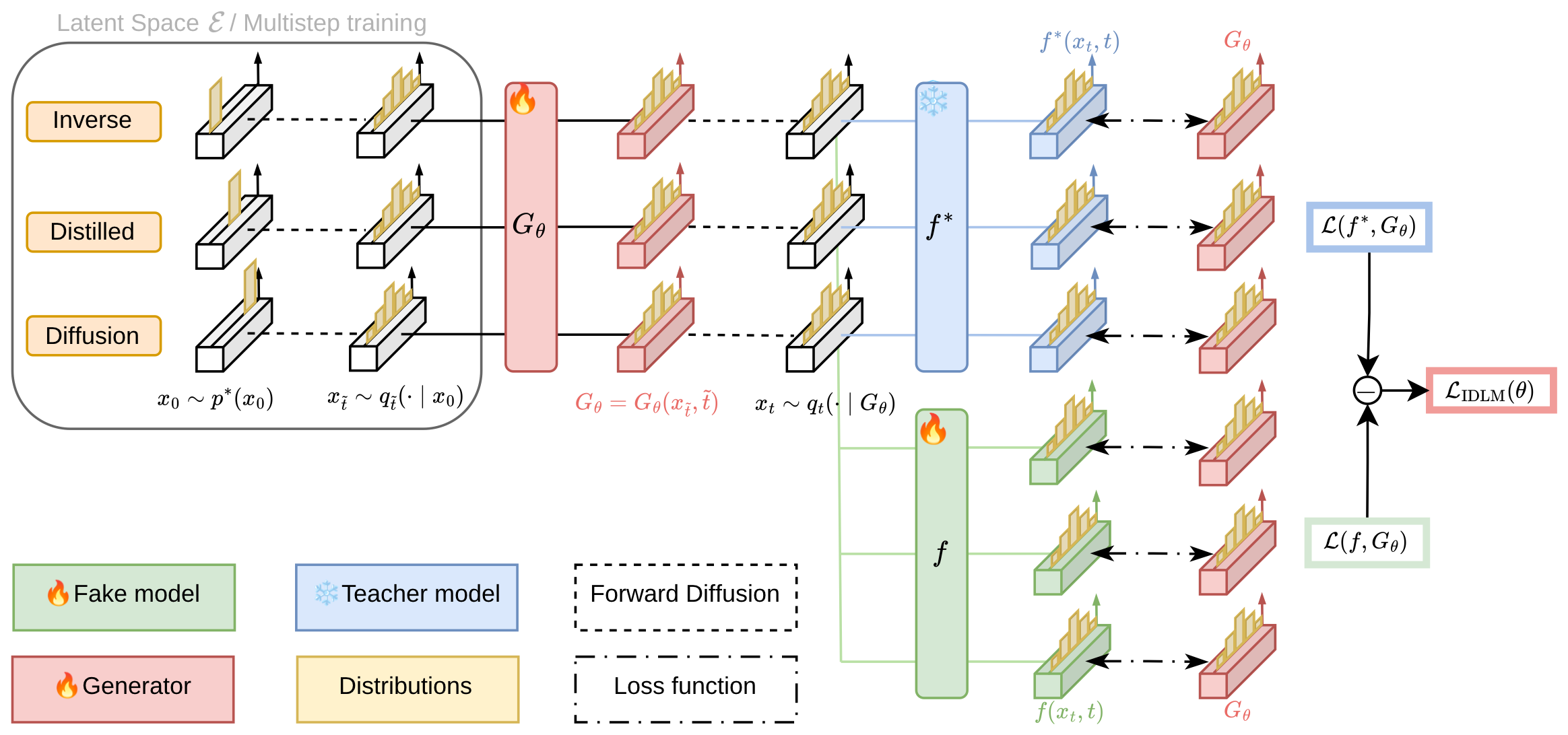
The practical training loop has two coupled parts. The student generator \(G_\theta\) defines the current distribution \(p_\theta\). The fake model \(f\) is then trained as an ordinary diffusion model on samples from this current student distribution. After this fake model has adapted to what the student currently produces, IDLM freezes \(f\) and updates \(G_\theta\) using the teacher-minus-fake gap:

Here \(f^\star\) is the frozen teacher trained on real data. The fake model \(f\) is trained on the current student samples, so it describes what the student already knows how to generate. During the generator update, both \(f^\star\) and \(f\) are fixed, and the parameters \(\theta\) are trained to minimize \(\mathcal{L}_{\mathrm{IDLM}}\). The first term is attractive: reducing \(\mathcal{L}(f^\star,p_\theta)\) encourages the student distribution to place probability on token choices that have small teacher loss. The second term is repulsive: because it is subtracted, the generator update minimizes \(-\mathcal{L}(f,p_\theta)\), equivalently maximizing \(\mathcal{L}(f,p_\theta)\) with \(f\) fixed. Therefore, tokens that are easy for the fake model but not consistently supported by the teacher are pushed down.

For MDLM, the \(\mathrm{SUBS}\) parameterization makes this particularly transparent. Revealed tokens are copied by both models, so they cancel out of the teacher-minus-fake difference. Only masked positions remain. At a masked position, let \(m\) denote the mask token and define the teacher-over-fake advantage vector \(a_t=\log f^\star(m,t)-\log f(m,t)\). Each coordinate \(a_{t,i}\) compares how much the teacher and fake model support vocabulary token \(i\) at time \(t\). The IDLM-MDLM loss becomes

Here \(G_\theta(\epsilon)\) is the student distribution over the vocabulary, while \(w_t\ge0\) is the time-dependent weight inherited from the masked-diffusion loss. The inner product \(\langle G_\theta(\epsilon),a_t\rangle\) is the student's current expected teacher-over-fake advantage. Since the loss is the negative of this quantity, minimizing it is equivalent to maximizing that expected advantage. Moving probability mass toward a token with larger \(a_{t,i}\) increases the inner product and decreases the loss, moving mass toward a token with smaller \(a_{t,i}\) has the opposite effect. If \(G_\theta(\epsilon)=\mathrm{softmax}(z_\theta)\), this becomes even sharper after taking the gradient with respect to the pre-softmax logit of token \(i\):

This equation makes the sign of the update explicit. Since \(w_t\ge0\) and \(G_{\theta,i}(\epsilon)>0\), gradient descent increases token \(i\)'s logit exactly when \(a_{t,i}\) is larger than the current average advantage \(\langle G_\theta(\epsilon),a_t\rangle\). The average term acts like a baseline: a token is attractive only if the teacher prefers it over the fake model more than the generator's current mixture does on average. Tokens below this baseline are pushed down, even if they still have some teacher probability. When \(f\) catches up with \(f^\star\) on student samples, \(a_t\approx0\), the bracket becomes zero, and the relative signal disappears.

3.5 Final Algorithm

In practice, one-step text generation is a difficult learning problem: the student would need to recover global structure and token-level details from a highly noisy state in a single jump. IDLM therefore trains the student as a few-step denoiser on a short reverse trajectory. In this practical parameterization, the latent variable is chosen to be \(\epsilon=(x_t,t)\): a noised state together with its diffusion time. At each training step, this pair is sampled from the forward process and passed to \(G_\theta\). The resulting prediction is evaluated under both \(f^\star\) and \(f\). The fake model minimizes the ordinary diffusion loss on the student distribution, while the generator minimizes the teacher-minus-fake objective. This alternating scheme implements the inverse-distillation signal without differentiating through an exact inner argmin.

The final IDLM training loop can be read as a simple two-model comparison: use the frozen teacher \(f^\star\) as a quality reference, train an auxiliary fake denoiser \(f\) to recognize the current student samples, and update the student generator \(G_\theta\) using the difference between the two losses. In other words, the fake model learns what the student is currently producing, while the student is pushed toward samples that the teacher explains better than the fake model.

Algorithm Train-IDLM(f_star, f, G_theta, data)
// f_star is frozen; f and G_theta are optimized.
repeat
    x0 ← sample(data)              // clean sequence
    t  ← Uniform(0, 1)             // diffusion time
    xt ← q_t(. | x0)               // forward noising

    x_hat ← G_theta(xt, t)        // student proposal

    // fake model: learn the student's current samples
    L_fake ← L_seq(f, x_hat)
    update f using L_fake

    // student: prefer teacher-supported samples
    L_idlm ← L_seq(f_star, x_hat) - L_seq(f, x_hat)
    update G_theta using L_idlm
until convergence

Algorithm Sample-IDLM(G_theta, process, K)
// A short grid replaces the long teacher chain.
tau_K, ..., tau_0 ← reverse_grid(K)
x_k ← terminal_noise(process)

for k = K, ..., 1 do
    x0_hat ← G_theta(x_k, tau_k)
             // predicted clean sequence

    x_k ← reverse_step(
        x_k, x0_hat, tau_k, tau_{k-1}
    )
             // MDLM mask step or Duo uniform step
end for

return x_k

The notation \(L_{\mathrm{seq}}\) denotes the sequence-level diffusion loss for the chosen teacher family. The training algorithm teaches \(G_\theta\) how to replace many small teacher denoising moves, and the sampling algorithm then reuses the same reverse process on a much shorter grid.

4. Results

def simple_math_problem() -> int:
    baseball_cost = 9 * 3
    basketball_cost = 8 * 14
    difference = basketball_cost - baseball_cost
    result = difference
    return result

def simple_math_problem() -> int:
    blue_car = 100
    red_car = blue_car * 0.60
    total_cost = blue_car + red_car
    result = total_cost
    return result

4.2 Unconditional generation on OpenWebText

OpenWebText is the main unconditional generation test: unlike TinyGSM, there is no clamped prompt, and the model must generate full \(1024\)-token sequences from the terminal noise distribution. We follow the prior DLM protocol: OpenWebText is tokenized with the GPT-2 tokenizer, documents are concatenated and wrapped with \(\texttt{eos}\) tokens, the final \(100{,}000\) documents are held out for validation, and sampling is evaluated in \(\texttt{float64}\) precision using the official Duo evaluation code. The question is how far we can compress pretrained teacher samplers: IDLM-MDLM replaces the \(1024\)-step MDLM teacher with \(16\) reverse steps, while IDLM-DCD pushes the greedy Duo-DCD teacher down to \(4\) steps. We report GenPPL from a fixed GPT-2 Large evaluator together with token entropy, but the main story is teacher acceleration under much smaller reverse-step budgets.

IDLM-MDLM \(16\) steps

GenPPL\(32.75\) Entropy\(5.42\)

… In the wake of angry remarks from the media, Sam Kicks Radio decided to take a shot, claiming that he had only ever learned how to get away with something bad. I want to get over it, he says, while the exchange returns to the same public dispute. …

IDLM-DCD^g \(4\) steps

GenPPL\(77.47\) Entropy\(5.28\)

… This device is not the only way to use features in this article. People who conduct interviews in secure environments are attracted by a two-way monitor, making it an ideal candidate for an interviewee who can adapt to secure systems. …

OpenWebText generation

Teacher IDLM student

Masked Diffusion

GenPPL ↓ 50 40 30 20 10 0

\(41.29\)

Teacher MDLM \(1024\) steps Entropy \(5.3\)

\(32.75\)

Student IDLM-MDLM \(16\) steps Entropy \(5.4\)

Distilled

Uniform Diffusion

GenPPL ↓ 80 60 40 20 0

\(71.72\)

Teacher \(\mathrm{Duo}^{g}\) \(1024\) steps Entropy \(5.2\)

\(68.04\)

Student \(\mathrm{IDLM\mbox{-}Duo}^{g}\) \(16\) steps Entropy \(5.6\)

\(77.47\)

Student \(\mathrm{IDLM\mbox{-}DCD}^{g}\) \(4\) steps Entropy \(5.3\)

Distilled

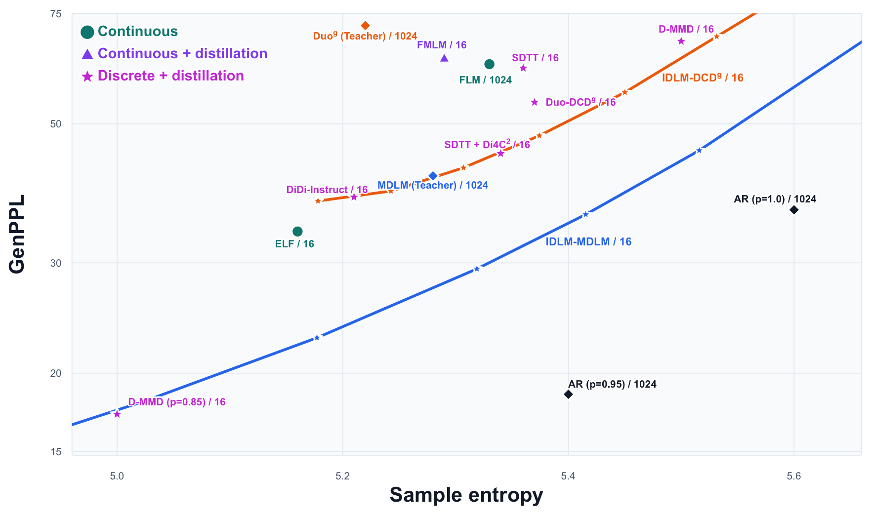
Although recent diffusion language models show strong unconditional generation quality, recent research discussions have emphasized that GenPPL should be interpreted together with diversity, since GenPPL is computed by an external language-model evaluator and changing the sampling temperature can move a method along an entropy-perplexity tradeoff, from lower-entropy samples with lower measured GenPPL to higher-entropy samples with higher measured GenPPL. The frontier view is therefore a way to ask a fairer question: at a comparable level of token entropy, which sampler achieves lower GenPPL?

In the frontier below, the desired direction is down and to the right: lower GenPPL while maintaining comparable or higher entropy. IDLM-MDLM at \(16\) steps lands on the strong masked-diffusion branch, improving over the \(1024\)-step MDLM teacher without moving into an obviously collapsed low-entropy regime. For uniform diffusion, the IDLM-DCD points show the main acceleration story: the \(16\)-step students remain in the competitive high-entropy region.

5. Conclusion

Diffusion language models offer parallel, bidirectional generation, but their long denoising chains make inference slow. An attractive approach is Inverse Distillation: instead of only shortening a reverse trajectory, it learns a fast student distribution whose induced diffusion training process remains compatible with the pretrained teacher. IDLM adapts this distribution-matching view to the language domain.

The result is a few-step generator with a clean target: match the teacher-supported data distribution. The theory gives a unique optimum, the practical method handles discrete non-smoothness, and the experiments show substantial step reductions on GSM8K and OpenWebText while keeping the teacher's quality.

6. BibTeX

@article{li2026idlm,
  title={IDLM: Inverse-distilled Diffusion Language Models},
  author={Li, David and Gushchin, Nikita and Abulkhanov, Dmitry and Moulines, Eric and Oseledets, Ivan and Panov, Maxim and Korotin, Alexander},
  journal={arXiv preprint arXiv:2602.19066},
  year={2026}
}